One of the things that I occasionally get frustrated by in sports statistics is the focus on estimates without presenting the associated uncertainty. While small sample size is often bandied about as an explanation for unusual results, one of the first things presented in statistics courses is the notion of a confidence interval. The simplest explanation of a confidence interval is that of a margin of error—you take the data and the degree of certainty you want, and it will give you a range covering likely values of the parameter you are interested in. It tacitly includes the sample size and gives you an implicit indication of how trustworthy the results are.

The most common version of this is the 95% confidence interval, which, based on some data, gives a range that will contain the actual value 95% of the time. For instance, say we poll a random sample of 100 people and ask them if they are right-handed. If 90 are right handed, the math gives us a 95% CI of (0.820, 0.948). We can draw additional sample and get more intervals; if we were to continue doing this, 95% of such intervals will contain the true percentage we are looking for. (How the math behind this works is a topic for another time, and indeed, I’m trying to wave away as much of it as possible in this post.)

One big caveat I want to mention before I get into my application of this principle is that there are a lot of assumptions that go into producing these mathematical estimates that don’t hold strictly in baseball. For instance, we assume that our data are a random sample of a single, well-defined population. However, if we use pitcher data from a given year, we know that the batters they face won’t be random, nor will the circumstances they face them under. Furthermore, any extrapolation of this interval is a bit trickier, because confidence intervals are usually employed in estimating parameters that are comparatively stable. In baseball, by contrast, a player’s talent level will change from year to year, and since we usually estimate something using a single year’s worth of data, to interpret our factors we have to take into account not only new random results but also a change in the underlying parameters.

(Hopefully all of that made sense, but if it didn’t and you’re still reading, just try to treat the numbers below as the margin of error on the figures we’re looking at, and realize that some of our interpretations need to be a bit looser than is ideal.)

For this post, I wanted to look at how much margin of error is in FIP, which is one of the more common sabermetric stats to evaluate pitchers. It stands for Fielding Independent Pitching, and is based only on walks, strikeouts, and home runs—all events that don’t depend on the defense (hence the name). It’s also scaled so that the numbers are comparable to ERA. For more on FIP, see the Fangraphs page here.

One of the reasons I was prompted to start with FIP is that a common modification of the stat is to render it as xFIP (x for Expected). xFIP recognizes that FIP can be comparatively volatile because it depends highly on the number of home runs a pitcher gives up, which, as rare events, can bounce around a lot even in a medium size sample with no change in talent. (They also partially depend on park factors.) xFIP replaces the HR component of FIP with the expected number of HR they would have given up if they had allowed the same number of flyballs but had a league average home run to fly ball ratio.

Since xFIP already embeds the idea that FIP is volatile, I was curious as to how volatile FIP actually is, and how much of that volatility is taken care of by xFIP. To do this, I decided to simulate a large number of seasons for a set of pitchers to get an estimate for what an actual distribution of a pitcher’s FIP given an estimated talent level is, then look at how wide a range of results we see in the simulated seasons to get a sense for how volatile FIP is—effectively rerunning seasons with pitchers whose talent level won’t change, but whose luck will.

To provide an example, say we have a pitcher who faces 800 batters, with a line of 20 HR, 250 fly balls (FB), 50 BB, and 250 K. We then assume that, if that pitcher were to face another 800 batters, each has a 250/800 chance of striking out, a 50/800 chance of walking, a 250/800 chance of hitting a fly ball, and a 20/250 chance of each fly ball being a HR. Plugging those into some random numbers, we will get a new line for a player with the same underlying talent—maybe it’ll be 256 K, 45 BB, and 246 FB, of which 24 were HR. From these values, we recompute the FIP. Do this 10,000 times, and we get an idea for how much FIP can bounce around.

For my sample of pitchers to test, I took every pitcher season with at least 50 IP since 2002, the first year for which the number of fly balls was available. I then computed 10,000 FIPs for each pitcher season and took the 97.5th percentile and 2.5th percentile, which give the spread that the middle 95% of the data fall in—in other words, our confidence interval.

(Nitty-gritty aside: One methodological detail that’s mostly important for replication purposes is that pitchers that gave up 0 HR in the relevant season were treated as having given up 0.5 HR; otherwise, there’s not actually any variation on that component. The 0.5 is somewhat arbitrary but, in my experience, is a standard small sample correction for things like odds ratios and chi-squared tests.)

One thing to realize is that these confidence intervals needn’t be symmetric, and in fact they basically never are—the portion of the confidence interval above the pitcher’s actual FIP is almost always larger than the portion below. For instance, in 2011 Bartolo Colon had an actual FIP of 3.83, but his confidence interval is (3.09, 4.64), and the gap from 3.83 to 4.64 is larger than the gap from 3.09 to 3.83. The reasons for this aren’t terribly important without going into details of the binomial distribution, and anyhow, the asymmetry of the interval is rarely very large, so I’m going to use half the length of the interval as my metric for volatility (the margin of error, as it were); for Colon, that’s (4.64 – 3.09) / 2 = 0.775.

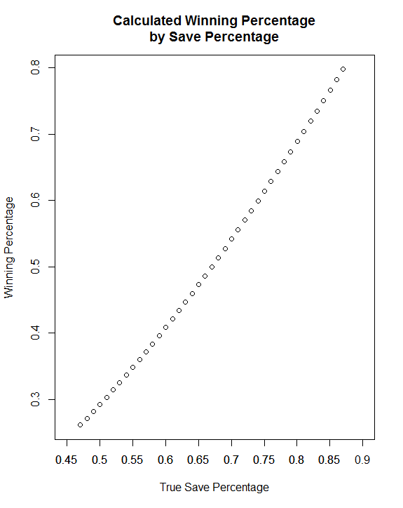
So, how big are these intervals? To me, at least, they are surprisingly large. I put some plots below, but even for the pitchers with the most IP, our margin of error is around 0.5 runs, which is pretty substantial (roughly half a standard deviation in FIP, for reference). For pitchers with only about 150 IP, it’s in the 0.8 range, which is about a standard deviation in FIP. A 0.8 gap in FIP is nothing to sneeze at—it’s the difference between 2013 Clayton Kershaw and 2013 Zack Greinke, or between 2013 Zack Greinke and 2013 Scott Feldman. (Side note: Clayton Kershaw is really damned good.)

As a side note, I was concerned when I first got these numbers that the intervals are too wide and overestimate the volatility. Because we can’t repeat seasons, I can’t think of a good way to test volatility, but I did look at how many times a pitcher’s FIP confidence interval contained his actual FIP from the next year. There are some selection issues with this measure (as a pitcher has to post 50 IP in consecutive years to be counted), but about 71% of follow-up season FIPs fall into the previous season’s CI. This may be a bit surprising, as our CI is supposed to include the actual value 95% of the time, but given the amount of volatility in baseball performance due to changes in skill levels, I would expect to see that the intervals diverge from actual values fairly frequently. Though this doesn’t confirm that my estimated intervals aren’t too wide, the magnitude of difference suggests to me it’s unlikely that that is our problem.

Given how sample sizes work, it’s unsurprising that the margin of error decreases substantially as IP increases. Unfortunately, there’s no neat function to get volatility from IP, as it depends strongly on the values of the FIP components as well. If we wanted to, we could construct a model of some sort, but a model whose inputs come from simulations seemed to me to be straying a bit far from the real world.

As I only want to see a rule of thumb, I picked a couple of round IP cutoffs and computed the average margin of error for every pitcher within 15 IP of that cutoff. The 15 IP is arbitrary, but it’s not a huge amount for a starting pitcher (2–3 starts) and ensures we can get a substantial number of pitchers included in each interval. The average FIP margin of error for pitchers within 15 IP of the cutoffs is presented below; beneath that is are scatterplots comparing IP to margin of error.

Note that due to construction I didn’t include anyone with less than 50 IP, and the most innings pitched in my sample is 266, so these cutoffs span the range of the data. I also looked at the median values, and there is no substantive difference.

This post has been fairly exploratory in nature, but I wanted to answer one specific question: given that the purpose of xFIP is to stabilize FIP, how much of FIP’s volatility is removed by using xFIP as an ERA estimator instead?

This can be evaluated a few different ways. First, the mean xFIP margin of error in my sample is about 0.54, while the mean FIP margin of error is 0.97; that difference is highly highly significant. This means there is actually a difference between the two, but looking at the average absolute difference of 0.43 is pretty meaningless—obviously a pitcher with an FIP margin of error of 0.5 can’t have a negative margin of error. Thus, we instead look at the percentage difference, which gives us the figure that 43% of the volatility in FIP is removed when using xFIP instead. (The median number is 45%, for reference.)

Finally, here is the above table showing average margins of error by IP, but this time with xFIP as well; note that the differences are all in the 42-48% range.

Thus, we see that about 45% of the FIP volatility is stripped away by using xFIP. I’m sort of burying the lede here, but if you want a firm takeaway from this post, there it is.

I want to conclude this somewhat wonkish piece by clarifying a couple of things. First, these numbers largely apply to season-level data; career FIP stats will be much more stable, though the utility of using a rate stat over an entire career may be limited depending on the situation.

Second, this volatility is not something that is unique to FIP—it could be applied to basically any of the stats that we bandy about on a daily basis. I chose to look at FIP partially for its simplicity and partially because people have already looked into its instability (hence xFIP); in the future, I’d like to apply this to other stats as well; for instance, SIERA comes to mind as something directly comparable to FIP, and since Fangraphs’ WAR is computed using FIP, my estimates in this piece can be applied to those numbers as well.

Third, the diminished volatility of xFIP isn’t necessarily a reason to prefer that particular stat. If a pitcher has an established track record of consistently allowing more/fewer HR on fly balls than the average pitcher, that information is important and should be considered. One alternative is to use the pitcher’s career HR/FB in lieu of league average, which gives some of the benefits of a larger sample size while also considering the pitcher’s true talent, though that’s a bit more involved in terms of aggregating data.

Since I got to rambling and this post is long on caveats relative to substance, here’s the tl;dr:

• Even if you think FIP estimates a pitcher’s true talent level accurately, random variation means that there’s a lot of volatility in the statistic.
• If you want a rough estimate for how much volatility there is, see the tables above.
• Using xFIP instead of FIP shrinks the margin of error by about 45%.
• This is not an indictment of FIP as a stat, but rather a reminder that a lot of weird stuff can happen in a baseball season, especially for pitchers.